How to learn representations under p4 and p4m symmetry groups
Published:
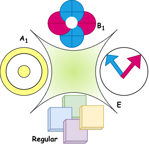
Building on the theoretical foundation presented in Beyond CNN: Chapter 0, Cohen and Welling brought the group-theoretic concepts directly into neural network architectures with their 2016 paper, “Group Equivariant Convolutional Networks”. While traditional CNNs natively handle translations, they fail to equivary with isometries like rotations and reflections. To solve this, they introduced group-equivariant convolutions (G-CNN), a natural generalization of convolutions that extends weight sharing beyond translations to include rotations, reflections, and other symmetries. G-CNN is a new type of layer that shares weights across a larger group of symmetries (specifically the p4 and p4m groups, representing 90-degree rotations and reflections). These layers effectively increased the expressive capacity of the network without adding any parameters.
Object and feature map
Domain \(\Omega\) (e.g. 2D \(\mathbb{Z}^2\) or 3D \(\mathbb{Z}^3\) Euclidean spaces) is an underlying space where we can define an object. An object can be an input image or a feature map generated within the intermediate layers of representation learning. We apply function space \(\mathbb{F}\) on domain \(\Omega\) to define object \(f\) (e.g. a 2D image or a protein 3D structure).
\[\mathbb{F}(\Omega, \mathbb{C})=\{f:\Omega \rightarrow \mathbb{C}\}\]where \(\mathbb{C} \in \mathbb{R}^K\) is the range of values taken by objects defined on \(\Omega\).
Equivariance and symmetry group
A function \(\Phi\) is equivariant to a transformation \(g\) if transforming the input and then applying \(\Phi\) gives the same result as applying \(\Phi\) first and then transforming the output:
\[\Phi(T_g x) = T'_g \Phi(x)\]Here \(T_g\) and \(T'_g\) are (possibly different) operators that represent the transformation \(g\) acting on the input and output spaces respectively.
You’ve already seen this with regular convolutions: shifting an image and then convolving gives the same result as convolving and then shifting. That’s just translation equivariance. The goal of G-CNNs is to make networks equivariant to a broader group of transformations \(G\).
Why equivariance and not invariance? Invariance means \(T'_g = I\) (the output doesn’t change at all). While that sounds useful, it’s actually too strong for intermediate layers. If your intermediate features are invariant to rotation, you’ve thrown away spatial information about where things are oriented, which makes it impossible to detect relative poses between features. Equivariance preserves structure; invariance destroys it.
A symmetry group is a set of transformations under which the properties of the object remain unchanged. A Group satisfies following properties:
- Has closure and can be composed (applying two transformations gives another transformation from the set)
- Has an identity (the “do nothing” transformation)
- Has inverses (every transformation can be undone)
The simplest example is the set of 2D integer translations, \(\mathbb{Z}^2\). A translation by \((n, m)\) composed with a translation by \((p, q)\) gives \((n+p, m+q)\). The inverse of \((n, m)\) is \((-n, -m)\). This is the group that regular CNNs exploit.
For more information see my previous post on this topic:
Equivariance and Invariance: The building blocks of geometric deep learning
Here we focus on two richer groups:
The group p4 p4 consists of all combinations of translations and 90-degree rotations in a grid. Every element can be written as a \(3 \times 3\) matrix:
\[g(r, u, v) = \begin{bmatrix} \cos(r\pi/2) & -\sin(r\pi/2) & u \\ \sin(r\pi/2) & \cos(r\pi/2) & v \\ 0 & 0 & 1 \end{bmatrix}\]where \(0 \leq r < 4\) (four rotations: 0°, 90°, 180°, 270°) and \((u, v) \in \mathbb{Z}^2\) are the translation components. Group composition is just matrix multiplication.
The group p4m p4m extends p4 with mirror reflections. Its elements are parameterized as:
\[g(m, r, u, v) = \begin{bmatrix} (-1)^m \cos\!\left(\tfrac{r\pi}{2}\right) & -(-1)^m \sin\!\left(\tfrac{r\pi}{2}\right) & u \\ \sin\!\left(\tfrac{r\pi}{2}\right) & \cos\!\left(\tfrac{r\pi}{2}\right) & v \\ 0 & 0 & 1 \end{bmatrix}\]where \(m \in \{0, 1\}\) controls the flip. This gives 8 distinct orientations (4 rotations × 2 flip states), making p4m a richer symmetry group.
Functions on domains vs functions on groups
In a regular CNN, a feature map (which is an object) is a function \(f : \mathbb{Z}^2 \to \mathbb{R}^K\) . It operates on a 2D grid of pixels (domain \(\mathbb{Z}^2\)) and at each pixel \((p, q)\) it assigns a \(K\)-dimensional vector of channels. A simple example is a grayscale image itself, which can be interpreted as a signal defined over the discrete grid (domain) \(\mathbb{Z}^2\), where each pixel contains a single intensity value (i.e., one channel). In CNN, each channel is generated by a filter. One channel might detect edges, another might detect textures, and another might detect corners. The only thing indexing the feature is the spatial position, so at each pixel we store features: \((p, q) \rightarrow\) feature vector.
In a G-CNN, feature maps become functions on the group \(G\) itself: \(f : G \to \mathbb{R}^K\). Instead of indexing by position alone, each feature is indexed by a full group element: a (position},rotation) pair for p4, or a (position, rotation, flip) triple for p4m. Therefore, for each transformation (like a rotation) AND position, we store features: (position, rotation) \(\rightarrow\) feature vector. Instead of just saying “there is an edge at (10, 5),” a G-CNN represents it as “there is an edge at (10, 5) with specific orientations (e.g., 30°, 90°, etc.),” explicitly encoding both position and transformation.
Group actions
When a transformation \(g \in G\) acts on a feature map \(f\), it does so by “pulling back” the coordinates of domain \(\mathbb{Z}^2\). Instead of moving each feature forward to a new location, we ask: “to know what the transformed feature map looks like at position \(x \in \mathbb{Z}^2\), which position in the original map should I look up?” That answer is \(g^{-1}x\):
\[[L_g f](x) = f(g^{-1} x)\]\(L_g\) is called the left action or left regular representation. It’s the operator that applies a group transformation \(g\) to a feature map by reindexing its domain coordinates.
The reason \(g^{-1}\) appears rather than \(g\) is a consistency requirement: applying transformation \(g\) and then \(h\) must equal applying \(gh\) in one shot. Using \(g^{-1}\) guarantees this — it makes \(L_g\) a proper group homomorphism (a structure-preserving map):
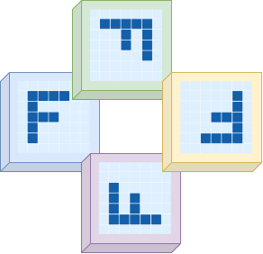
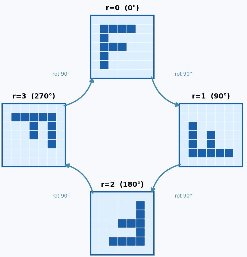
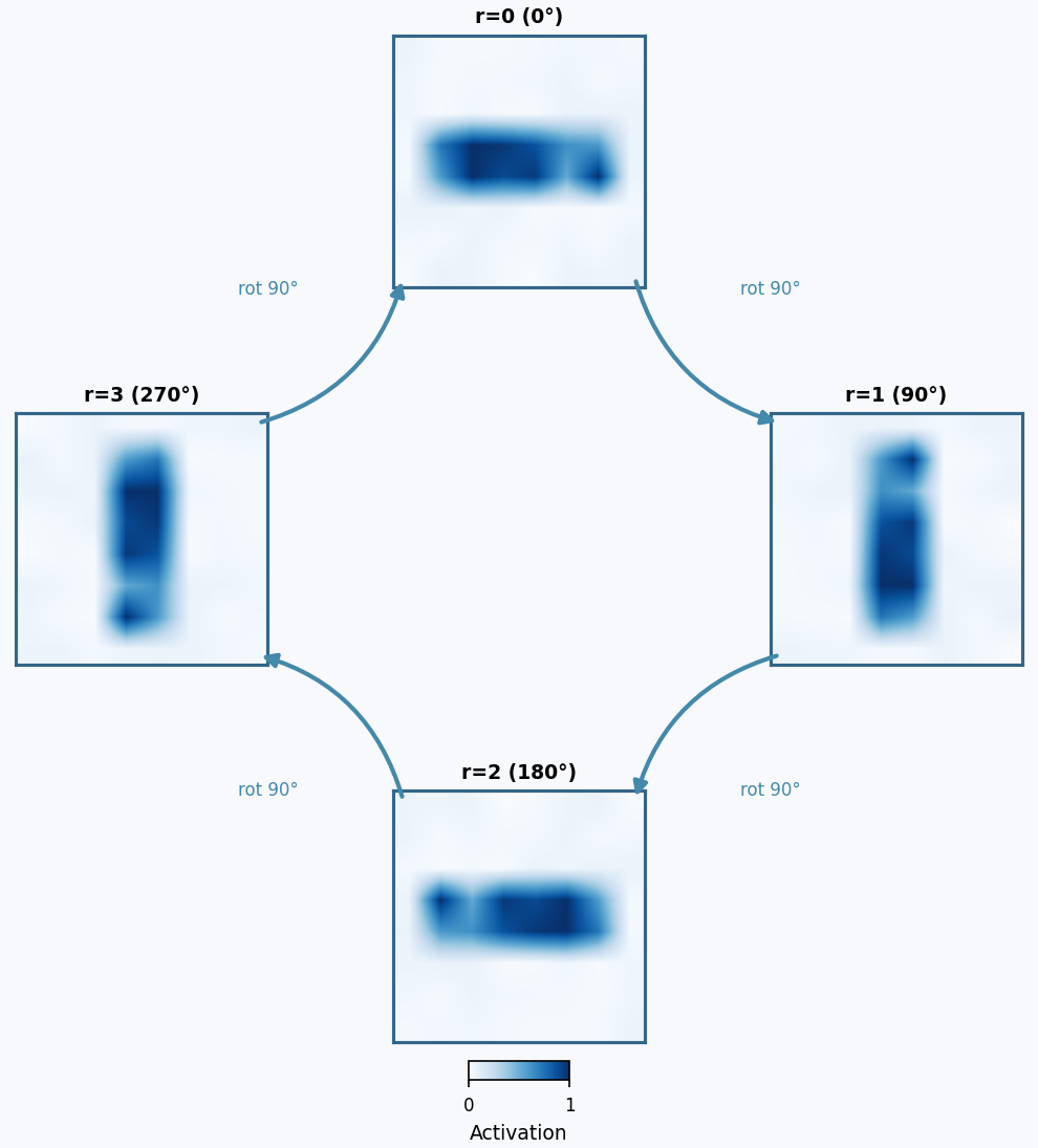
\[\begin{aligned} &[L_g f](x) = f(g^{-1} x) \\ &[L_g L_h f](x) = L_g(L_h f)(x) = (L_h f)(g^{-1} x) = f\!\left(h^{-1}(g^{-1} x)\right) \\ &(gh)^{-1} = h^{-1} g^{-1} \\ &f\!\left(h^{-1} g^{-1} x\right) = f\!\left((gh)^{-1} x\right) = [L_{gh} f](x)\\ &gh \mapsto L_{gh} = L_g L_h \\ \end{aligned}\]To visualize a p4 feature map, imagine four copies of a 2D spatial grid arranged in a circle, one per rotation. When you rotate such a feature map, each copy shifts to the next position and its contents rotate by 90°. This interplay between the “rotation index” and the spatial content is exactly what the group structure captures.
Standard CNNs fail at rotation equivariance
In a regular CNN, the correlation of a feature map \(f\) with the convolutional filter \(\psi\) is:
\[[f \star \psi](x) = \sum_{y \in \mathbb{Z}^2} \sum_{k=1}^{K} f_k(y)\, \psi_k(y - x)\]where \(y\) ranges over all pixel positions, \(k\) ranges over the \(K\) input channels, \(f_k(y)\) is the feature map value at pixel \(y\) in channel \(k\), and \(\psi_k(y - x)\) is the weight of filter \(\psi\) at the relative offset \((y - x)\) in channel \(k\). The output at location \(x\) is a weighted sum of the neighborhood around \(x\). As you know this is the standard convolution.
For translations, this operation is equivariant: shift the input by \(t\) pixels, and the output shifts by exactly \(t\) pixels:
\[\begin{aligned} &[L_t f](y) = f(y - t) \\ &[[L_t f] \star \psi](x) = \sum_{y \in \mathbb{Z}^2} \sum_{k=1}^{K} f_k(y - t)\, \psi_k(y - x) \\ &y' = y - t \Rightarrow y = y' + t \\ &[[L_t f] \star \psi](x) = \sum_{y' \in \mathbb{Z}^2} \sum_{k=1}^{K} f_k(y')\, \psi_k((y' + t) - x) \\ &[[L_t f] \star \psi](x) = \sum_{y' \in \mathbb{Z}^2} \sum_{k=1}^{K} f_k(y')\, \psi_k(y' - (x - t)) \\ &[[L_t f] \star \psi](x) = [f \star \psi](x - t) \\ &[[L_t f] \star \psi](x) = [L_t (f \star \psi)](x) \\ \end{aligned}\]But for a rotation \(r\), things break down. Working through the same algebra with a rotation gives:
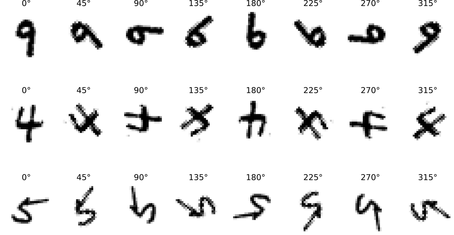
\[\begin{aligned} &[L_r f](y) = f(r^{-1} y) \\ &[[L_r f] \star \psi](x) = \sum_{y \in \mathbb{Z}^2} \sum_{k=1}^{K} f_k(r^{-1} y)\, \psi_k(y - x) \\ &y' = r^{-1} y \Rightarrow y = r y' \\ &[[L_r f] \star \psi](x) = \sum_{y' \in \mathbb{Z}^2} \sum_{k=1}^{K} f_k(y')\, \psi_k(r y' - x) \\ &x = r(r^{-1} x) \\ &r y' - x = r y' - r(r^{-1} x) = r(y' - r^{-1} x) \\ &\psi_k(r(y' - r^{-1} x)) \\ &[L_{r^{-1}} \psi](z) = \psi(r z) \\ &\psi_k(r(y' - r^{-1} x)) = [L_{r^{-1}} \psi]_k(y' - r^{-1} x) \\ &[[L_r f] \star \psi](x) = \sum_{y' \in \mathbb{Z}^2} \sum_{k=1}^{K} f_k(y')\, [L_{r^{-1}} \psi]_k(y' - r^{-1} x) \\ &[[L_r f] \star \psi](x) = [f \star (L_{r^{-1}} \psi)](r^{-1} x) \\ &[[L_r f] \star \psi](x) = [L_r (f \star (L_{r^{-1}} \psi))](x) \\ \end{aligned}\]Notice the extra \(L_{r^{-1}} \psi\) on the right. This says: rotating the input and then convolving with \(\psi\) is equivalent to convolving with the already-rotated filter \(L_{r^{-1}}\psi\) and then rotating the output. The filter on the right-hand side has changed. It’s now the \(r\) degree-rotated version of the original $\psi$. So convolving with the same unmodified \(\psi\) on both sides gives different results. The operation is not equivariant to rotation.
This is why a standard CNN that wants to detect a feature in all four orientations (in case of p4 group) needs to learn four separate filters. G-CNNs solve this by sharing weights across all orientations.
G-Convolutions
The G-CNN replaces the standard convolution with a G-correlation, which explicitly correlates over all transformations in \(G\).
First layer
In the first layer, both the input \(f\) and the filter \(\psi\) are ordinary functions on \(\mathbb{Z}^2\). The G-correlation produces a feature map that is a function on \(G\):
\[[f \star \psi](g) = \sum_{y \in \mathbb{Z}^2} \sum_{k=1}^{K} f_k(y)\, \psi_k(g^{-1} y)\]The output is indexed by elements \(g \in G\). For each \(g\), the value \([f \star \psi](g)\) is obtained by applying the transformation \(g^{-1}\) to the filter and computing its inner product with the input. As a result, the feature map is a function defined on the group \(G\), rather than on \(\mathbb{Z}^2\).
Subsequent layers
After the first layer, each feature map is no longer just a grid over \(\mathbb{Z}^2\), but a function on the group \(G\).
\[f : G \to \mathbb{R^K}\]Instead of assigning a value to each spatial location, it assigns a value to each transformation \(g \in G\) (for example, a combination of a translation and a rotation). In typical settings, \(G\) may be a product such as \(G = \mathbb{Z}^2 \rtimes C_n\). In this case, an element \(g\) can be written as \(g = (x, r)\), where \(x \in \mathbb{Z}^2\) encodes a translation and \(r \in C_n\) encodes a discrete rotation. A feature map \(f\) therefore assigns a vector \(f(g)\) to each transformation \(g\), rather than to each position alone.
Because of this change in representation, filters must be defined in the same space. A filter \(\psi\) is therefore also a function on \(G\), so that it can be compared meaningfully with the input feature map at every group element.
\[\psi : G \to \mathbb{R^K}\]Intuitively, both the input and the filter now describe patterns indexed by transformations rather than just positions.
For example, if \(G = \mathbb{Z}^2\), a feature map is a standard image-like grid. If \(G = \mathbb{Z}^2 \times C_4\), where \(C_4\) represents four rotations, then a feature map assigns a value to each location \((x,y)\) and each orientation \(r \in \{0^\circ, 90^\circ, 180^\circ, 270^\circ\}\). In this case, the filter must also specify a response for each position and orientation, so that it can detect not only where a pattern appears, but also in which orientation it appears.
The generalized correlation operator is then defined by comparing the input with transformed versions of the filter over all elements \(g \in G\):
\[[f \star \psi](g) = \sum_{h \in G} \sum_{k=1}^{K} f_k(h)\, \psi_k(g^{-1} h)\]This is similar to a standard convolution, except the “spatial domain” is now the group \(G\) itself.
Proving equivariance
The equivariance proof follows the same substitution trick as we saw before, now using \(h' = u^{-1}h\) (left multiplication by \(u\) is a bijection on G):
\[\begin{aligned} {}[[L_u f] \star \psi](g) &= \sum_{h \in G} \sum_{k=1}^{K} f_k(u^{-1}h)\, \psi_k(g^{-1}h) \\ &= \sum_{h' \in G} \sum_{k=1}^{K} f_k(h')\, \psi_k(g^{-1}uh') \\ &= \sum_{h' \in G} \sum_{k=1}^{K} f_k(h')\, \psi_k((u^{-1}g)^{-1}h') \\ &= [L_u[f \star \psi]](g) \end{aligned}\]So the G-correlation commutes with \(L_u\) for any \(u \in G\). The network is fully equivariant.
Everything else is equivariant too
Equivariance isn’t just a property of the G-convolution layer. It propagates cleanly through all the other components of a modern network.
Pointwise nonlinearities
Let \(\nu : \mathbb{R} \to \mathbb{R}\) be a nonlinearity (e.g. ReLU). The operator $C_\nu$ applies $\nu$ pointwise:
\[(C_\nu f)(g) = \nu(f(g))\]It changes values independently at each \(g \in G\) without mixing locations.
Group transformations act by shifting the input function: \((L_h f)(g) = f(h^{-1}g)\). A key property is that these two operations commute: \(C_\nu L_h f(g) = \nu(f(h^{-1}g)) = L_h C_\nu f(g)\). This means applying a group transformation and then a nonlinearity gives the same result as applying the nonlinearity first and then transforming. Therefore, pointwise nonlinearities preserve equivariance. Here is the proof:
\[\begin{aligned} (C_\nu L_h f)(g) &= C_\nu(L_h f)(g) \\ &= \nu((L_h f)(g)) \\ &= \nu(f(h^{-1}g)). \end{aligned}\] \[\begin{aligned} (L_h C_\nu f)(g) &= (C_\nu f)(h^{-1}g) \\ &= \nu(f(h^{-1}g)). \end{aligned}\]Since both expressions are equal for all \(g \in G\), we conclude: \(C_\nu L_h f = L_h C_\nu f\). ReLU, sigmoid, tanh: they’re all equivariant for free.
Pooling
We define max-pooling over a neighborhood \(U \subset G\) as:
\[(Pf)(g) = \max_{u \in U} f(u),\]We show that pooling commutes with the group action.
\[\begin{aligned} (P L_h f)(g) &= \max_{u \in U} (L_h f)(u) \\ &= \max_{u \in U} f(h^{-1}u). \end{aligned}\]Now substitute \(u = hu'\), which preserves the set structure:
\[\begin{aligned} (P L_h f)(g) &= \max_{u' \in h^{-1}U} f(u') \\ &= (P f)(h^{-1}g) \\ &= (L_h P f)(g). \end{aligned}\]Therefore, \(P L_h f = L_h P f\)
So pooling is equivariant.
If pooling is taken over the entire group (e.g. all four rotations of p4) at each spatial location then the output will be a rotation-invariant feature map which is useful at the final layer if you want a fully invariant prediction. However, doing this too early (at intermediate layers) hurts performance, because it discards pose information before the network has had a chance to use it.
Batch normalization and residual connections
Batch normalization and residual connections are commonly used in CNNs. \textbf{Question:} Do you think they are also equivariant? Why?
Putting it all together
G-CNN isn’t that different from a standard network in structure: you simply replace each convolution with a G-convolution, adjust the number of channels to keep parameters in check, and let the network carry orientation-aware feature maps through its layers, optionally pooling over them at the end for invariance. But this small change leads to a much bigger shift in perspective: instead of treating features as unstructured vectors, the network now respects the symmetries of the problem by design. As a result, it doesn’t have to relearn the same pattern in multiple orientations, making it more sample-efficient, more expressive with the same number of parameters, and more reliable in how it generalizes.