How group convolutional networks exploit symmetry

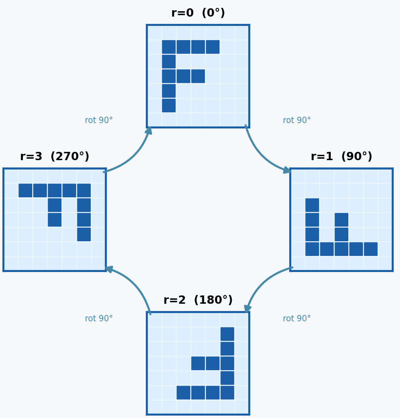
In the previous post How to learn representations under p4 and p4m symmetry groups we saw how a G-CNN extends ordinary convolution. It shares one filter across a group of transformations such as the four 90-degree rotations in \(p4\). For a \(p4\) G-CNN, a feature at each pixel has four orientation channels. When the image rotates by 90 degrees, those channels cycle to new positions. Therefore if the input rotates or flips, the internal features change in a known, predictable and useful way.

A quick recap on symmetry, equivariance and invariance

When people first hear about symmetry, they often think about invariance: if the input rotates, the output stays the same. That is useful at the very end of a predictive model, where we only care about the class label. But inside a deep network, we usually don’t want to throw away pose information too early. Later layers still need to know whether an edge is vertical, horizontal, or diagonal. A filter \(\psi\) is equivariant if transforming the input and then applying the network gives the same result as applying the network first and then transforming the features:

It says the feature changes predictably when the input changes. Once we know the transformation \(g\), we know exactly how the feature response should change. We do not need to learn a separate filter from examples. Here, \(f\) is the input signal or feature map, \(g\) is a transformation such as a rotation or reflection, \(\psi \in \Psi\) is the learnable filter, \(\rho(g)\) is a representation on how the input transforms, and \(\pi(g)\) is a representation on how the feature transforms.

G-CNNs: stacks of transformations

The basic transformation law is:

It says the value that ends up at position \(x\) after a transformation \(g\) comes from the old position \(g^{-1}x\).

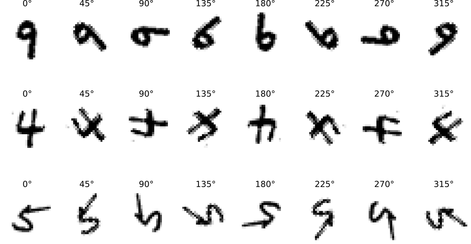
For translations, standard convolution is already equivariant. If you shift the image, the feature map shifts in the same way. This is one of the big reasons CNNs work so well. But standard CNNs don’t naturally know what to do with rotations and reflections. Data augmentation helps, but the architecture itself still treats each pose as something it may need to learn again. G-CNNs fix this by using a group such as \(p4\) or \(p4m\). They explicitly track position and orientation, so a rotated input produces a rotated feature map with its orientation channels permuted in a predictable way.

Instead of learning only one filter, G-CNN applies all transformed versions of the filter:

The resulting filter tensor contain an additional group dimension:

where \(H\) and \(W\) are the spatial size of the kernel, \(C_{in}\) and \(C_{out}\) are the number of input and output channels and \(\|G\|\) is the number of transformations in the group \(G\). For example, a rotation-equivariant CNN with 8 discrete orientations stores \(C \times 8\) feature maps corresponding to the different orientations. Although it’s expressive, it makes every feature pay the cost of carrying a full orientation stack.

What does G-CNN learn?

In G-CNN, the network learns only a single base filter \(\psi\). The remaining filters are generated automatically by applying the group transformations:

\(\psi\), as a convolution filter, is a function defined over spatial positions \(\psi:\mathbb{R}^{2}\rightarrow\mathbb{R}\) and \(x\) represents a spatial coordinate inside the filter kernel. \(g^{-1}\) maps the transformed coordinate back to the original coordinate.

For example, for a discrete rotation group \(p4\) \(G=\{0^\circ,90^\circ,180^\circ,270^\circ\}\) the filter bank becomes \(\{\psi_0,\psi_{90},\psi_{180},\psi_{270}\}\). A \(3\times3\) learned filter can be represented as:

where \(a,\ldots,i\) are learned parameters. The group transformation learns only one filter and then deterministically generates transformed versions of the original filter by changing the spatial coordinates. A \(90^\circ\) rotation produces:

The rotated filter is therefore not an additional learned parameter. It is obtained directly from the original filter through the group operation. Therefore, a G-CNN learns only the base filter \(\psi\). The symmetry group automatically generates the set of transformed filters without requiring additional trainable parameters.

From input space to group feature space in G-CNNs

In a standard CNN, the input image is transformed into a feature map:

where \(x\) represents the spatial position, \(X(x)\) is the input value, and \(F(x)\) is a feature vector at that position.

The output feature map tenosr has the form:

where \(C\) is the number of channels and \(H\) and \(W\) are the spatial dimensions.

In a G-CNN, the first layer is different. Instead of producing only spatial features, the network produces features that are indexed by both spatial position and transformation state:

The resulting feature map tensor becomes:

For example, for the discrete rotation group \(p4\)

each spatial location contains a set of orientation-dependent features:

Thus, a feature is not only associated with a spatial location, but also with a transformation state.

The first layer of G-CNN: Lifting convolution

The first layer of a G-CNN is called a lifting convolution. It maps the input image space to a feature space that includes the group dimension. Instead of the standard convolution:

the lifting convolution computes:

where the filters are generated from the base filter through the group action:

The output therefore belongs to a space that combines spatial and transformation dimensions:

The network has learned a base filter \(\psi\), while the transformed filters \(\psi_g\) are generated deterministically by the symmetry operations.

Subsequent layers of G-CNN

After the first layer, the input is no longer a standard feature map. It is a feature field defined over both spatial positions and transformation states: \(F(x,g)\)

Subsequent layers perform group convolutions that combine information from neighboring spatial positions and different transformation states. The group convolution is defined as:

The term \(g^{-1}h\) ensures that the relationship between different orientations is treated consistently under the group transformation.

Towards Steerable CNNs

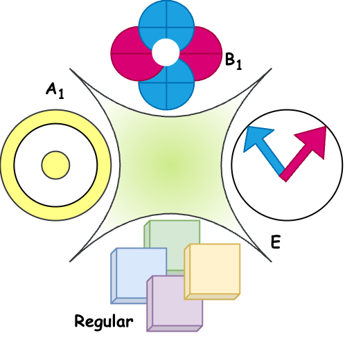
Although G-CNN is a real improvement over conventional CNNs, it raises an important question: must every feature be stored as a full stack of orientations?