Diffusion: Forward process
Published:
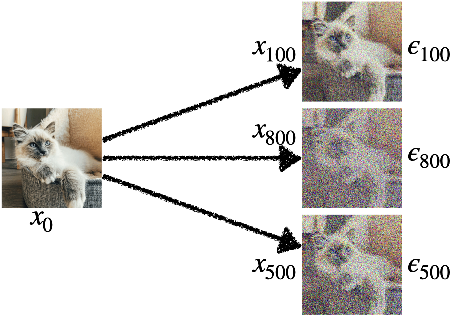
To train a diffusion model, we first need to add noise to our samples (e.g. an image or a 3D protein structure) and then train a model to predict the noise. The process of adding noise is called forward process.
How to add noise?
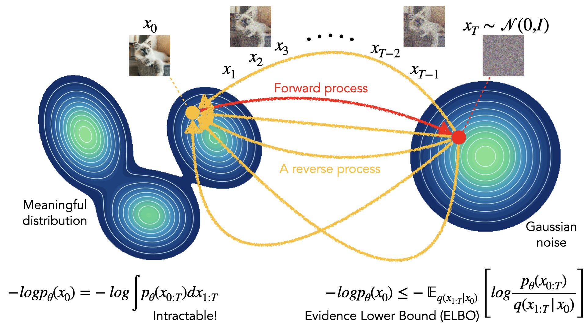
In the forward process the objective is to add noise to the observed noiseless data until we reach a standard Gaussian (normal) distribution \(\mathcal{N}(0, I)\). \(I\) is the covariance matrix. For example, for an \(8 \times 8\) image, the covariance matrix is of size \(64 \times 64\) representing the relationships between all the pixels.
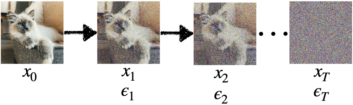
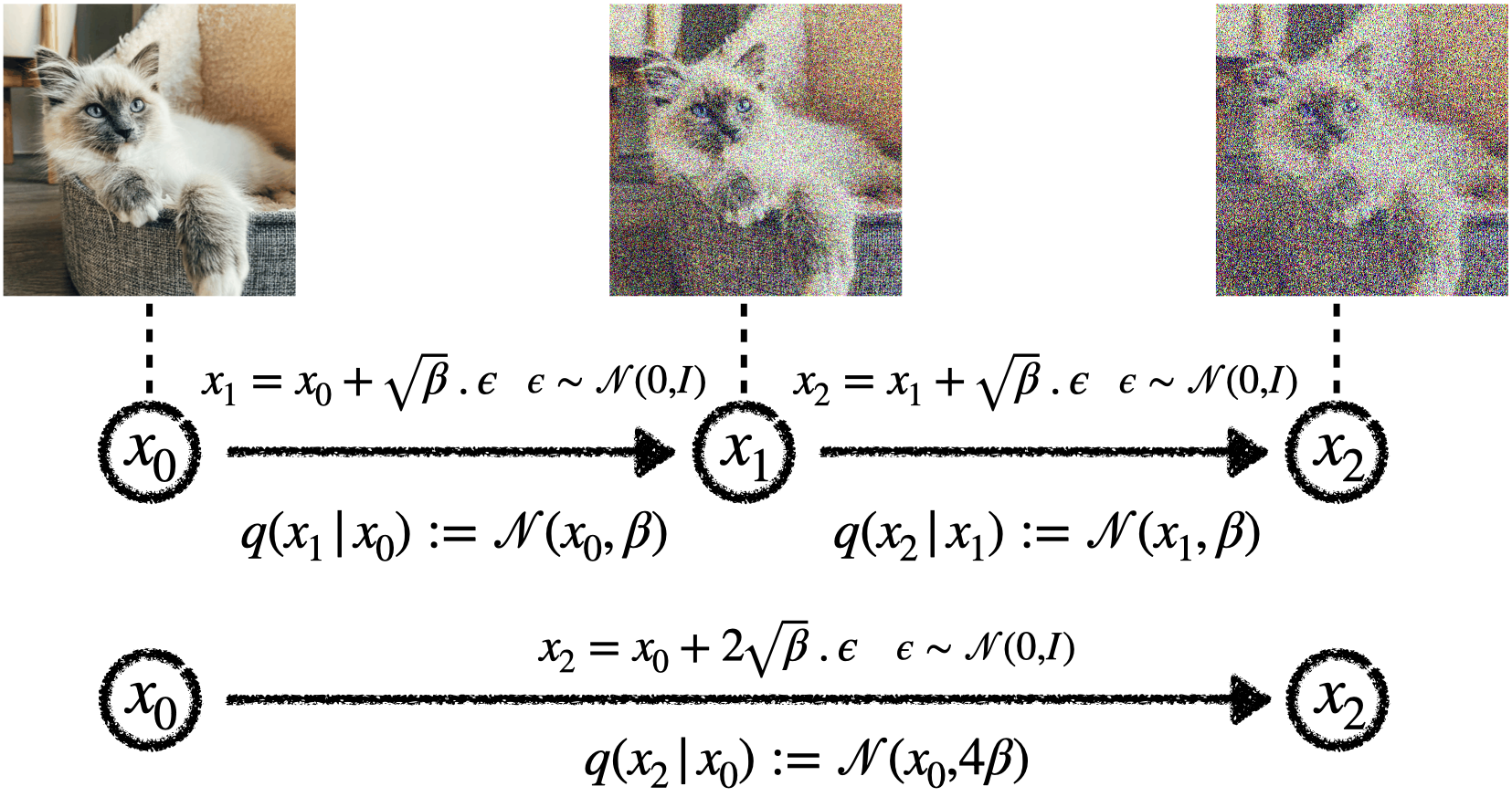
This noise is a fraction of a random variable \(\epsilon\) that follows a standard normal distribution: \(\epsilon \sim \mathcal{N}(0, I)\). To obtain the noisy data at time step \(t=1\), we can either add the noise to the clean noiseless data at time step \(t=0\) or simply sample from a conditional normal distribution \(q(x_1 \rvert x_0) := \mathcal{N}(x_0,\beta)\), centered at \(x_0\), with variance \(\beta\).
The same concept applies to the next step:
Calculate \(x_2 = x_1 + \sqrt{\beta}.\epsilon\) or sample from \(q(x_2 \rvert x_1) := \mathcal{N}(x_1,\beta)\).
Alternatively we can jump from time step \(t=0\) to time step \(t=2\) directly by combining the equations above:
Calculate \(x_2 = x_0 + 2\sqrt{\beta}.\epsilon\) or sample from \(q(x_2 \rvert x_0) := \mathcal{N}(x_0,4\beta)\).
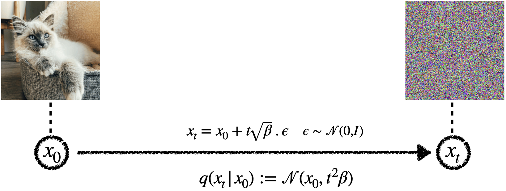
We can jump directly to any time step \(t\) by either calculating \(x_t = x_0 + t\sqrt{\beta}.\epsilon\) or sampling from \(q(x_t \rvert x_0) := \mathcal{N}(x_0,t^2\beta)\).
Can we reach a standard Gaussian distribution?
However, when \(t\) approaches infinity, we don’t achieve our goal of reaching a standard Gaussian distribution \(q(x_t \rvert x_0) := \mathcal{N}(x_0,t^2\beta) \neq \mathcal{N}(0,I)\). The mean is not 0 and the variance increases indefinitely.
Therefore, we redefine the way we add noise at each step \(t-1\) to obtain \(x_t\):
\[x_t = \sqrt{1-\beta}x_{t-1} + \sqrt{\beta}.\epsilon \qquad \epsilon \sim \mathcal{N}(0,I)\]This is equivalent to sampling from conditional distribution
\[\qquad q(x_t \rvert x_{t-1}) := \mathcal{N}(x_t; \sqrt{1-\beta}\,x_{t-1}, \beta I)\]Also, instead of using a constant variance \(\beta\), we can define a noise schedule and have different variances for different time steps: \(\beta_1 < \beta_2 < \cdots < \beta_T\).
\[x_t = \sqrt{1-\beta_t}x_{t-1} + \sqrt{\beta_t}.\epsilon_t \qquad \epsilon_t \sim \mathcal{N}(0,I)\] \[q(x_t \rvert x_{t-1}) := \mathcal{N}(x_t; \sqrt{1-\beta_t}\,x_{t-1}, \beta_t I)\]This way, early steps add a tiny amount of noise, while later steps add more noise.
The complete forward process
The complete forward process is a trajectory containing all the intermediate noisy states \(x_1,\cdots,x_T\) conditioned on \(x_0\). We represent this trajectory using a joint conditional distribution \(q(x_1,\cdots,x_T \mid x_0)\). To determine this joint distribution, we use the chain rule of probability to decompose it into individual conditional distributions. Then, we assume a first-order Markov chain, in which each noising step depends only on the previous state.
\[\begin{aligned} &q(x_1,\cdots,x_T|x_0) = q(x_{1:T} | x_0) = \\ &q(x_1 | x_0) q(x_2 | x_1, x_0) \cdots q(x_T | x_{T-1}, \cdots, x_0) = \\ &q(x_1 | x_0) q(x_2 | x_1) \cdots q(x_T | x_{T-1}) = \\ &\prod_{t=1}^T q(x_t | x_{t-1}) \end{aligned}\]Jump directly to time step \(t\)
Given this new definition, can we jump directly from \(x_0\) to any time step \(t\), obtaining \(x_t\): \(q(x_t \rvert x_0) \xrightarrow{t \to \infty} \mathcal{N}(0,I)\)? In other words, can we find a function \(f\) for this direct jump:
\[x_t \overset{?}{=} f(x_0) \qquad q(x_t \rvert x_0) := ?\]To achieve this, we use two new variables \(\alpha_t = 1-\beta_t\) and \(\bar\alpha_t = \prod_{s=1}^t\alpha_s\).
Now let’s write \(x_1\), \(x_2\), and \(x_3\) in terms of the previous steps:
\[\begin{aligned} x_1 &= \sqrt{1-\beta_1}x_{0} + \sqrt{\beta_1}.\epsilon_1 \\ \\ x_2 &= \sqrt{1-\beta_2}x_{1} + \sqrt{\beta_2}.\epsilon_2 \\ &= \sqrt{1-\beta_2}\left(\sqrt{1-\beta_1}x_{0} + \sqrt{\beta_1}.\epsilon_1\right) + \sqrt{\beta_2}.\epsilon_2 \\ &= \sqrt{(1-\beta_2)(1-\beta_1)}x_0 + \sqrt{(1-\beta_2)\beta_1}\epsilon_1 + \sqrt{\beta_2}\epsilon_2 \\ &= \sqrt{\alpha_2\alpha_1}x_0 + \sqrt{\alpha_2\beta_1}\epsilon_1 + \sqrt{\beta_2}\epsilon_2 \\ \\ x_3 &= \sqrt{1-\beta_3}x_{2} + \sqrt{\beta_3}.\epsilon_3 \\ &= \sqrt{\alpha_3}\left( \sqrt{\alpha_2\alpha_1}x_0 + \sqrt{\alpha_2\beta_1}\epsilon_1 + \sqrt{\beta_2}\epsilon_2 \right) + \sqrt{\beta_3}\epsilon_3 \\ &= \sqrt{\alpha_3\alpha_2\alpha_1}x_0 + \sqrt{\alpha_3\alpha_2\beta_1}\epsilon_1 + \sqrt{\alpha_3\beta_2}\epsilon_2 + \sqrt{\beta_3}\epsilon_3 \\ &= \sqrt{\bar{\alpha}_3}x_0 +\sqrt{\alpha_3\alpha_2\beta_1}\epsilon_1 +\sqrt{\alpha_3\beta_2}\epsilon_2 +\sqrt{\beta_3}\epsilon_3 \\ &= \sqrt{\bar{\alpha}_3}x_0 +\sqrt{\alpha_3\alpha_2(1-\alpha_1)}\epsilon_1 +\sqrt{\alpha_3(1-\alpha_2)}\epsilon_2 +\sqrt{1-\alpha_3}\epsilon_3 \end{aligned} \qquad \epsilon_1,\epsilon_2,\epsilon_3 \sim \mathcal{N}(0,I)\]We can deduce the form of \(x_t\):
\[x_t = \sqrt{\bar{\alpha}_t}\,x_0 + \sum_{i=1}^{t} \sqrt{(1-\alpha_i)\prod_{j=i+1}^{t}\alpha_j}\,\epsilon_i \qquad \epsilon_i \sim \mathcal{N}(0,I), i.i.d\]Since \(x_t\) is an affine combination of independent and identically distributed Gaussian variables, it is also a Gaussian conditioned on \(x_0\): \(x_t \rvert x_0 \sim \mathcal{N}\left(\mu,\sigma^2\right)\). Therefore:
\[x_t = \sqrt{\bar{\alpha}_t}\,x_0 + \sum_{i=1}^{t} \sqrt{(1-\alpha_i)\prod_{j=i+1}^{t}\alpha_j}\,\epsilon_i \qquad \epsilon_i \sim \mathcal{N}(0,I), i.i.d \qquad \operatorname{Var}[\epsilon_i] = I\] \[x_t = \sqrt{\bar{\alpha}_t}\,x_0 + \sum_{i=1}^{t} C_i\epsilon_i\]From the equation above, the mean of \(x_t\) is \(\mathbb{E}[x_t \rvert x_0] = \sqrt{\bar{\alpha}_t}x_0\). Its covariance is:
\[\begin{aligned} \operatorname{Cov}[x_t \rvert x_0] &= \operatorname{Cov}\left(\sum_{i=1}^{t} C_i\epsilon_i|x_0\right) \\ &=\operatorname{Cov}\left(\sum_{i=1}^{t} C_i\epsilon_i\right) \\ &=\sum_{i=1}^{t}\operatorname{Cov}\left(C_i\epsilon_i\right) =\sum_{i=1}^{t}C^2_i\operatorname{Var}[\epsilon_i] = \sum_{i=1}^{t}C^2_i I \\ &= \left(\sum_{i=1}^{t}(1-\alpha_i)\prod_{j=i+1}^{t}\alpha_j\right)I \end{aligned}\]Using the telescoping method:
\[\begin{aligned} \sum_{i=1}^{t}(1-\alpha_i)\prod_{j=i+1}^{t}\alpha_j &= (1-\alpha_1)\prod_{j=2}^{t}\alpha_j +(1-\alpha_2)\prod_{j=3}^{t}\alpha_j +\cdots +(1-\alpha_t) \\ &= \left(\prod_{j=2}^{t}\alpha_j-\prod_{j=1}^{t}\alpha_j\right) +\left(\prod_{j=3}^{t}\alpha_j-\prod_{j=2}^{t}\alpha_j\right) +\cdots +(1-\alpha_t) \\ &= 1-\prod_{j=1}^{t}\alpha_j \\ &= 1-\bar{\alpha}_t \end{aligned}\]In summary:
\[\mathbb{E}[x_t \rvert x_0] = \sqrt{\bar{\alpha}_t}x_0 \qquad \operatorname{Cov}[x_t | x_0] = (1-\bar{\alpha}_t)I\]And therefore the mapping formula that we were looking for is:
\[x_t = \sqrt{\bar\alpha_t}x_0 + \sqrt{(1-\bar\alpha_t)}.\epsilon \qquad \epsilon \sim \mathcal{N}(0,I)\]Or equivalently:
\[q(x_t \rvert x_0) := \mathcal{N}(x_t; \sqrt{\bar\alpha_t}\,x_0, (1-\bar\alpha_t)I)\]We can see that \(x_t\) converges to a standard normal distribution when \(t\) approaches infinity: \(q(x_t \rvert x_0) \xrightarrow{t \to \infty} \mathcal{N}(0,I)\)
The forward process creates a training dataset of noisy images
During training, we randomly select a time step \(t\) and add noise to an original image using the formula derived above. This allows us to generate noisy images at different noise levels without applying the noise steps sequentially. The model learns to predict the noise added to each image, which can later be used to remove the noise during the reverse process.