Diffusion: Reverse process
Published:
Quick recap of the forward process
One noisy step:
\[q(x_t|x_{t-1}) := \mathcal{N}(x_t; \sqrt{1-\beta_t}\,x_{t-1}, \beta_t I)\]Jump to an arbitrary time step \(t\):
\[q(x_t|x_0) := \mathcal{N}(x_t; \sqrt{\bar\alpha_t}\,x_0, (1-\bar\alpha_t)I)\]Complete forward process:
\[\begin{aligned} &q(x_1,\cdots,x_T|x_0) = q(x_{1:T} | x_0) = \\ &q(x_1 | x_0) q(x_2 | x_1, x_0) \cdots q(x_T | x_{T-1}, \cdots, x_0) = \\ &q(x_1 | x_0) q(x_2 | x_1) \cdots q(x_T | x_{T-1}) = \\ &\prod_{t=1}^T q(x_t | x_{t-1}) \end{aligned}\]where \(x_0\) is the observed data, \(x_1,\cdots,x_{T-1}\) form a sequence of latent noisy states, and \(x_T\) follows the terminal distribution, chosen to be approximately standard Gaussian: \(x_T \sim \mathcal{N}(0, I)\).
One denoising step
The reverse process is the opposite of the forward process. It performs denoising to remove the noise from the data step by step:
\[x_T \rightarrow x_{T-1} \rightarrow \cdots \rightarrow x_1 \rightarrow x_0\]Let’s assume there is a probability density function \(p_\theta\), called approximate posterior, that allows us to reverse the individual noising steps: \(x_{t} \rightarrow x_{t-1}\).
While the forward process is defined by a conditional Gaussian distribution q(x_t \rvert x_{t-1}) with mean \(\sqrt{1-\beta_t}\,x_{t-1}\) and variance \(\beta_t I\), the reverse process depends on the learnable parameters \(\theta\), which are optimized during training to effectively remove the noise. We can define a single denoising step p_\theta(x_{t-1} \rvert x_t) as a Gaussian distribution.
\[p_\theta(x_{t-1} | x_t) := \mathcal{N}(x_{t-1}; \mu_\theta(x_t, t), \Sigma_\theta(x_t, t))\] 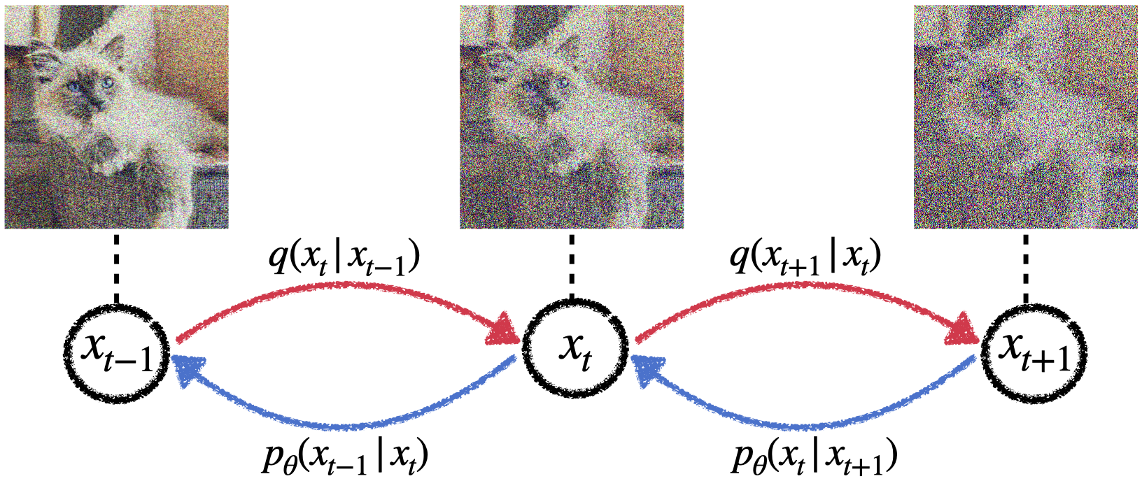
The mean of this Gaussian distribution is \(\mu_\theta(x_t, t)\) and its variance is \(\Sigma_\theta(x_t, t)\). Both are functions parameterized by \(\theta\) and depend on the current noisy state \(x_t\) and time step \(t\).
Complete reverse process
Similar to the forward process, the complete reverse process describes a trajectory containing all the intermediate denoised states \(x_T,\cdots,x_1\) starting at \(x_T\). We represent this trajectory using a joint distribution \(p_\theta(x_T,\cdots,x_0)\). To determine this joint distribution, we use the chain rule of probability to decompose it into individual conditional distributions. We then assume a first-order Markov chain, in which each noising step depends only on the previous state.
\[p_\theta(x_T,\cdots,x_0) = p_\theta(x_{0:T}) := p(x_T)\prod_{t=1}^T p_\theta(x_{t-1}|x_t)\] 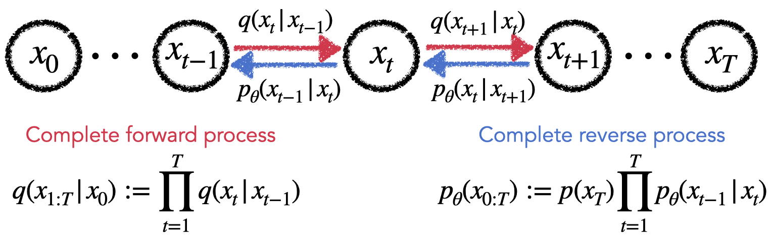
How to optimize parameters \(\theta\)?
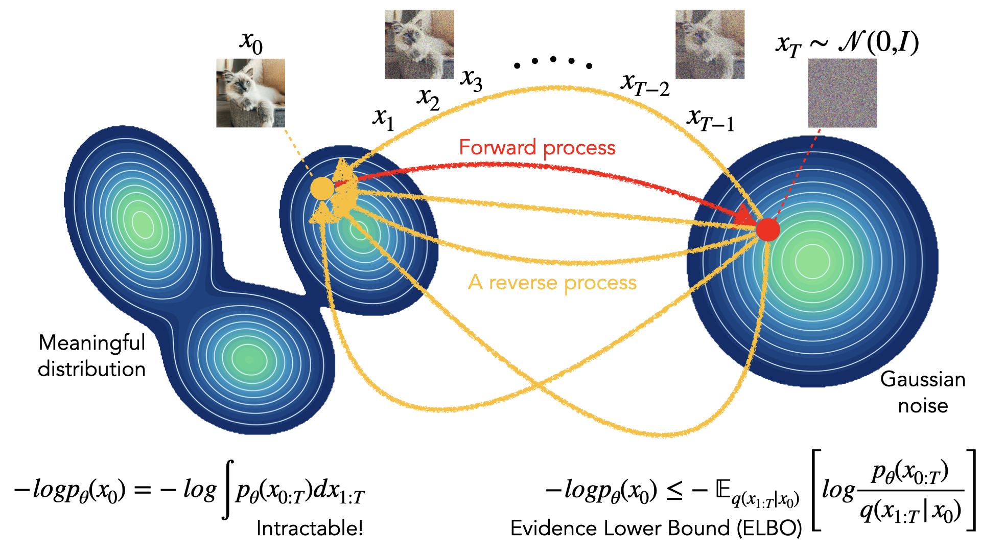
To find the best \(\theta\) that explains the observed data \(x_0\), we need to minimize the negative log-likelihood (or maximize the log-likelihood) computed by marginalizing over all possible intermediate noisy states \(x_1, \ldots, x_T\):
\[-logp_\theta(x_0) = -log\int p_\theta(x_{0:T})dx_{1:T}\]In other words, over all possible latent trajectories connecting \(x_T\) to \(x_0\). Of course, trajectories must follow a specific Markov factorization for both
complete forward process (red path):
\[q(x_{1:T} | x_0) := \prod_{t=1}^T q(x_t | x_{t-1}) \qquad q(x_t|x_{t-1}) := \mathcal{N}(x_t; \sqrt{1-\beta_t}\,x_{t-1}, \beta_t I)\]and complete reverse process (blue path):
\[p_\theta(x_{0:T}) := p(x_T)\prod_{t=1}^T p_\theta(x_{t-1}|x_t) \qquad p_\theta(x_{t-1} | x_t) := \mathcal{N}(x_{t-1}; \mu_\theta(x_t, t), \Sigma_\theta(x_t, t))\]With many diffusion steps, this high-dimensional marginalization becomes intractable. The likelihood requires integrating over the high-dimensional continuous latent trajectory.
So, instead of directly maximizing the exact likelihood, we find and optimize a tractable lower bound on it, called the Evidence Lower Bound, or ELBO:
\[logp_\theta(x_0) \geq \mathbb{E}_{q(x_{1:T} | x_0)}\left[log \frac{p_\theta(x_{0:T})}{q(x_{1:T} | x_0)}\right]\]